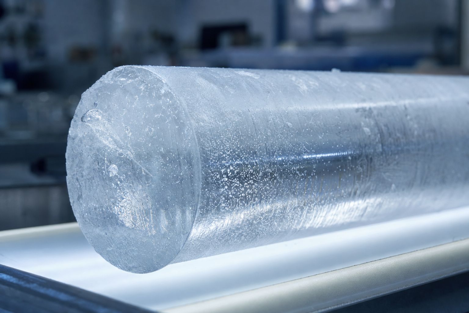
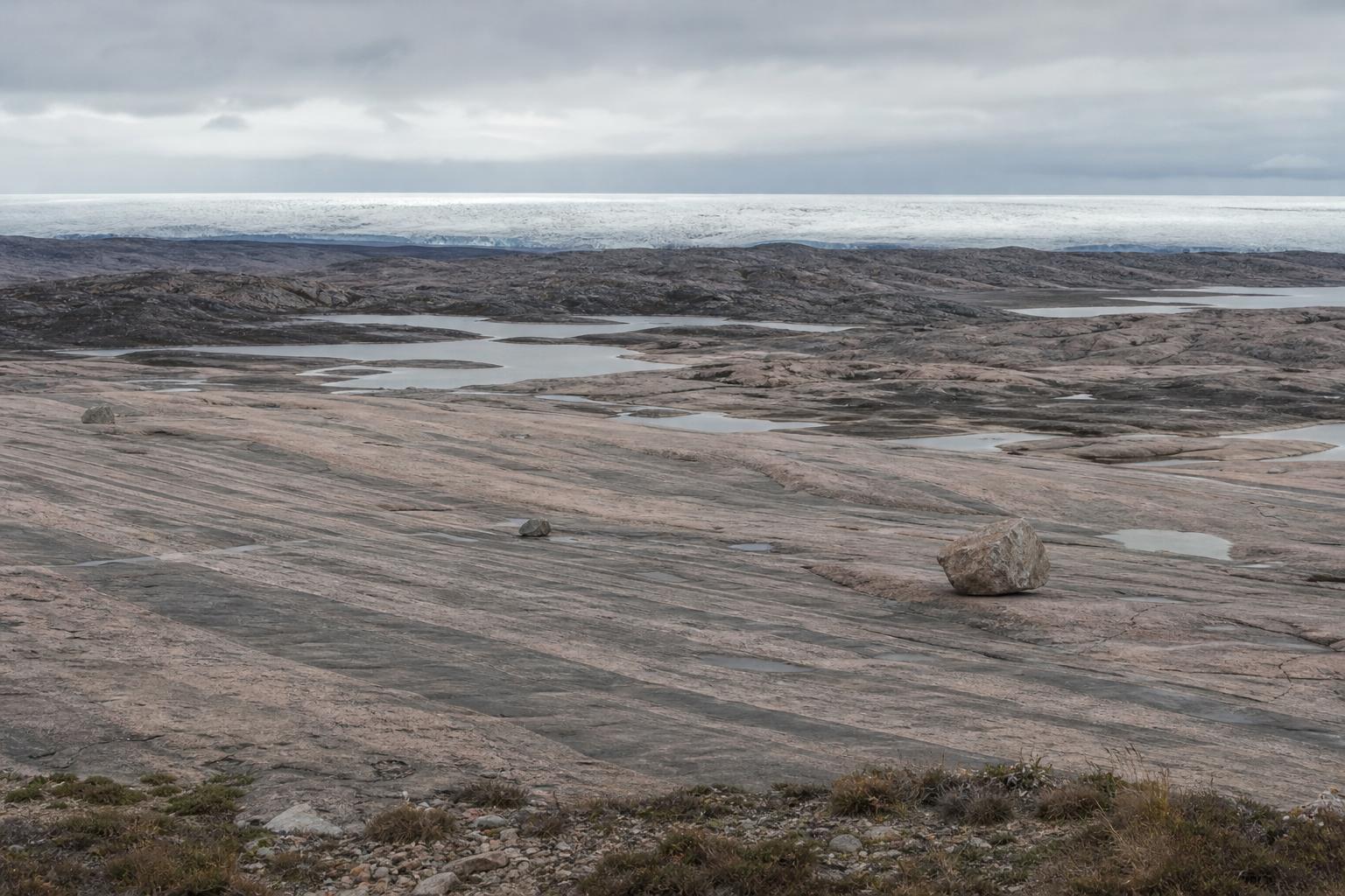
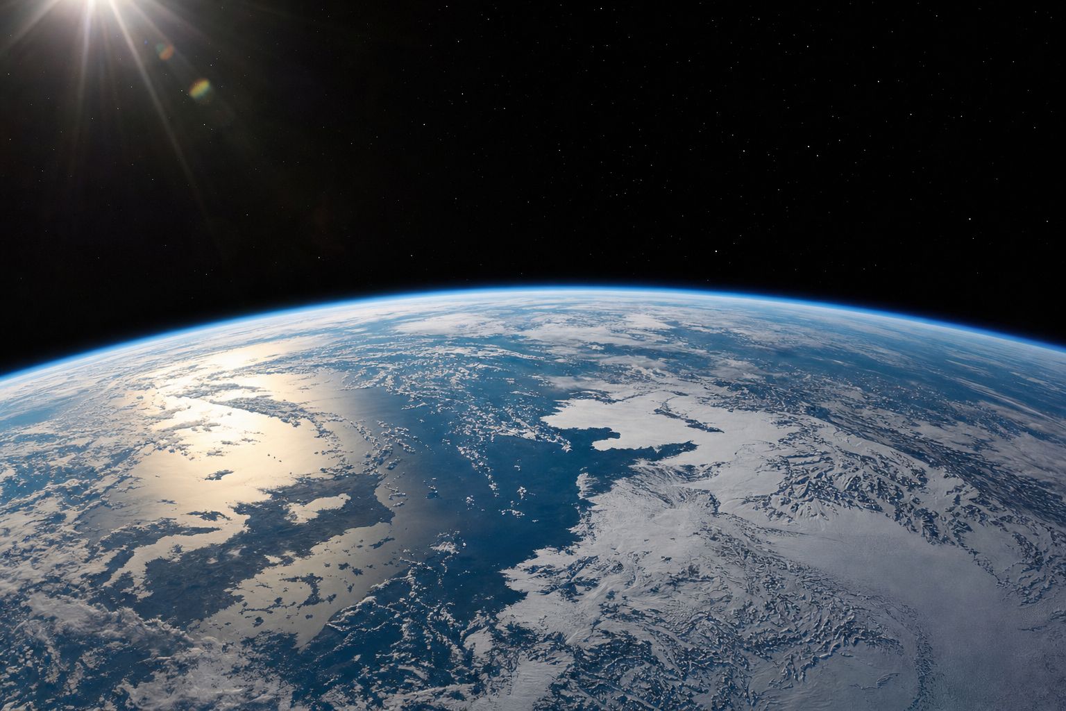
This week two studies looked at old ice: one suggests part of Tibet's Guliya ice cap is more than 128,000 years old, another offers an ocean model for why carbon dioxide fell in past ice ages. This film explains the fundamentals behind them: how Louis Agassiz read the idea of an ice age in boulders, what the world looked like 21,000 years ago when the Gulf of Thailand was dry land, how three slow changes in Earth's orbit and tilt change summer sunshine in the north, how Milutin Milanković calculated them, how ocean mud proved him right in 1976, how ice and carbon dioxide amplify a small nudge, what is still unexplained, and why today's warming is not orbital.
Interactive 3D film10 minThe last 2.6 million yearsPublished 31 October 2026
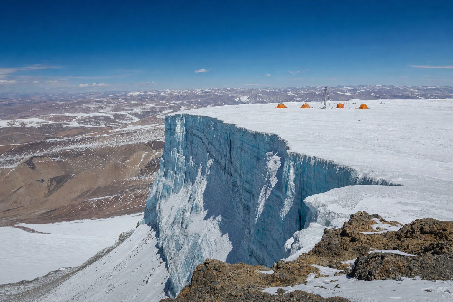
On the Guliya ice cap, high on the Tibetan Plateau, the ice may be more than a hundred and twenty-eight thousand years old, a new study suggests.
Ice that old has lived through the end of an ice age. Again and again, for two and a half million years, ice sheets have grown and melted. What sets the rhythm?
A high ice cap A drill camp on a remote Tibetan ice cap. AI-generated still.
128,000+
years: the team’s estimate for the oldest ice
41,000+
years ago: a magnetic-field event used as a marker
Guliya, dated anew (Ohio State, 2026)
Boulders in the wrong place
When the Gulf of Thailand was dry
Three slow changes in the orbit
Proof from the sea floor, and CO2
In this film
Prologue
Two new looks at old ice
Ohio State University (30 September 2026), on a study in Science Advances led by Lonnie Thompson: dating with beryllium and chlorine isotopes, using the Laschamp geomagnetic excursion more than 41,000 years ago as a marker, suggests the record of the Guliya ice cap in northwestern Tibet may reach back well over 128,000 years; earlier work had placed its start in the mid-Holocene. ScienceDaily (28 October 2026), on Shankle and colleagues at the University of St Andrews in the Journal of Climate: in idealized ocean simulations, cooling only the far north drew down 74% as much CO2 as cooling the whole planet; the authors call it a plausible mechanism, not a confirmed cause.
The 3D scenes are simplified teaching models: the orbit is exaggerated, ice and coastlines are drawn approximately, and the curves are schematic unless a source is named.
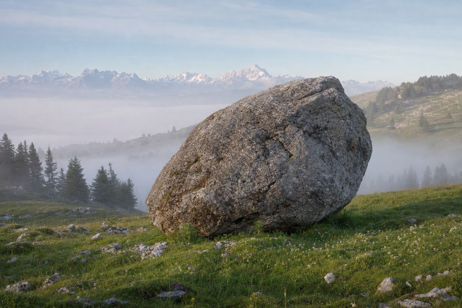
The idea is younger than you might think. On the limestone hills of the Swiss Jura lie huge granite boulders that do not match the rock beneath them. How did they get there?
In July 1837, at a meeting in Neuchâtel, the naturalist Louis Agassiz gave a startling answer: ice. Great sheets of ice had once covered the land and carried the rocks there.
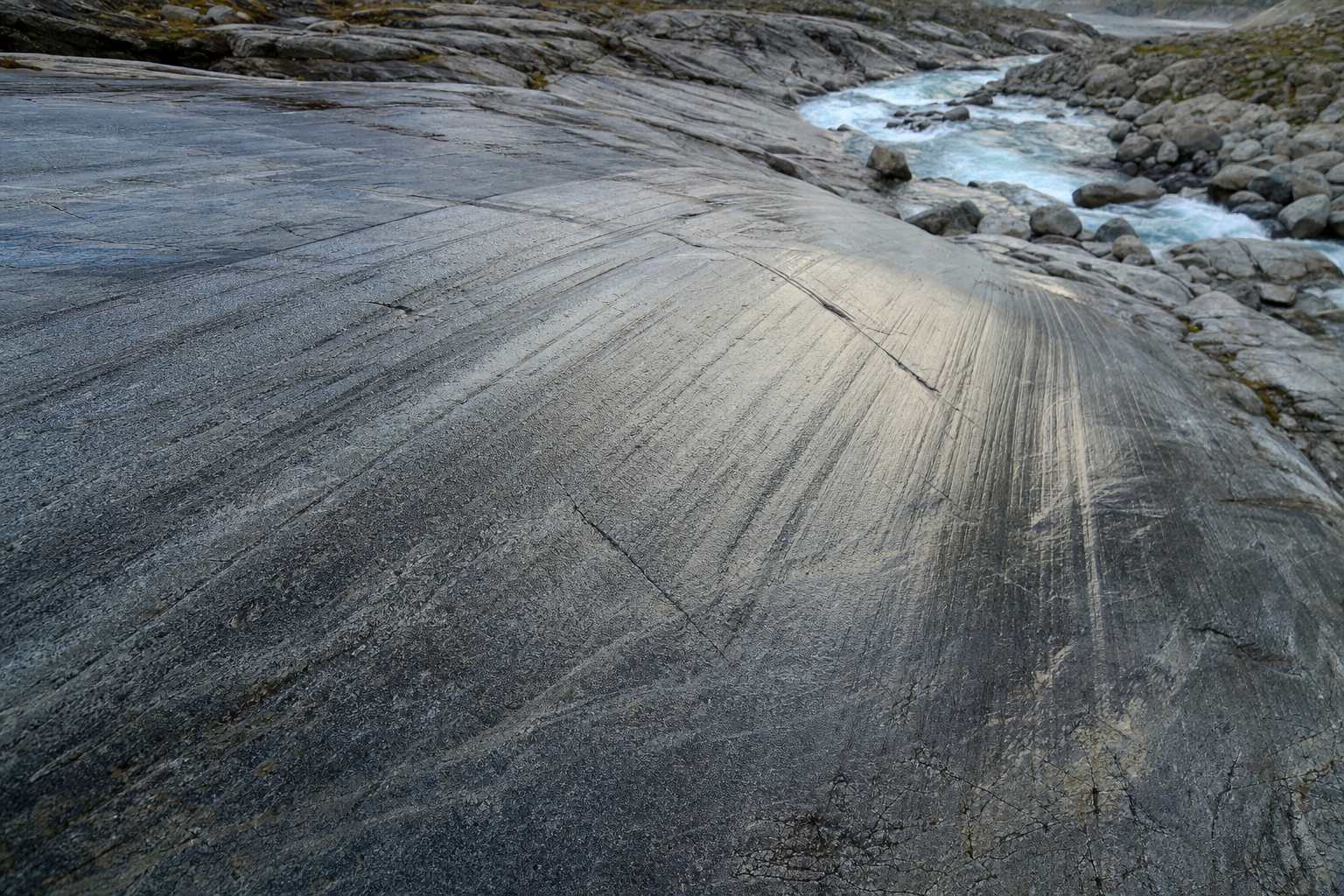
Polished, scratched bedrock and long ridges of rubble called moraines told the same story. In 1840 he set out the evidence in Studies on Glaciers: the world had lived through an ice age.
A glacial erratic A lone granite block on a limestone pasture. AI-generated still.
24 July 1837 Agassiz’s address in Neuchâtel
1838 On the erratic blocks of the Jura
1840 Études sur les glaciers
An idea takes shape
Erratics: boulders far from their bedrock
Polished rock with parallel scratches
Moraines: ridges of dumped rubble
What ice leaves behindGlacial striations Bedrock scratched by stones dragged under moving ice. AI-generated still.
Chapter I · The idea of an ice age
Agassiz and the erratic boulders
Ships Education, on Agassiz: on 24 July 1837, as president of the Swiss Society of Natural Sciences, Louis Agassiz gave the opening address in Neuchâtel and, instead of the customary review, presented evidence for past glaciation; he argued that erratic blocks, polished and striated rock and moraines were best explained by ice, not floods or drifting ice floes; his paper on the erratic blocks of the Jura followed in 1838 and Études sur les glaciers in 1840, ahead of Jean de Charpentier’s monograph on Alpine glaciation.
The 3D scenes are simplified teaching models: the orbit is exaggerated, ice and coastlines are drawn approximately, and the curves are schematic unless a source is named.
Today we know the cold came not once but again and again. Since the Quaternary period began two point five eight million years ago, ice sheets have grown and melted across the northern continents many times.
The cold phases are called glacials and the warm ones interglacials. We live in a warm one, the Holocene, which began about eleven thousand seven hundred years ago; in everyday speech, the ice age means the last glacial.
2.58 million
years ago: it begins, with ice spreading in the north
11,700
years ago: the Holocene begins
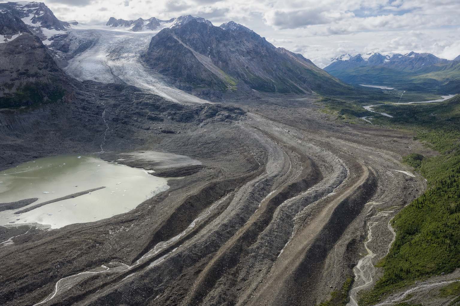
The QuaternaryWhat a glacier leaves Curving moraine ridges below a valley glacier. AI-generated still.
Geology: any time with ice sheets, including now
Everyday: the last glacial period
Glacial: a cold phase; interglacial: a warm one
Two meanings of “ice age”
Antarctica
the largest, around the South Pole
Greenland
the only one left in the north
Ice sheets left today
Chapter I · The idea of an ice age
Glacials and interglacials
Wikipedia, Quaternary: the period began about 2.58 million years ago (its base was redefined in 2009), marking the onset of Northern Hemisphere glaciation; ice sheets grew and shrank cyclically; the Holocene, the current interglacial, began about 11,700 years ago when the last glacial period ended.
The 3D scenes are simplified teaching models: the orbit is exaggerated, ice and coastlines are drawn approximately, and the curves are schematic unless a source is named.
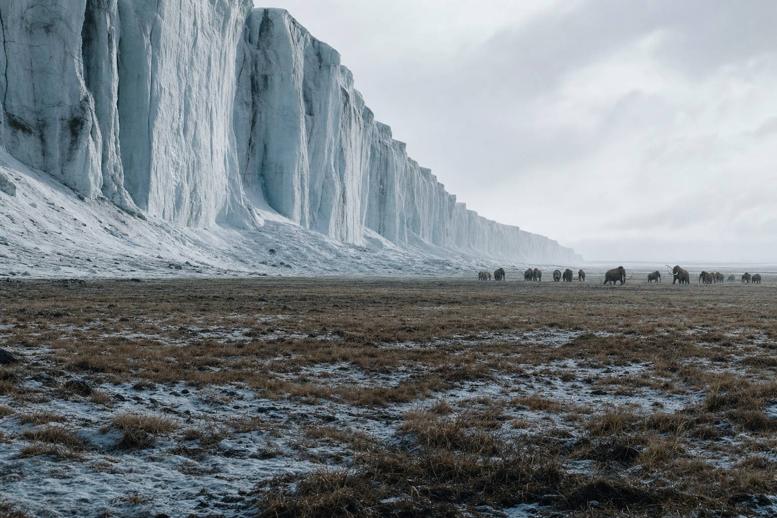
The last glacial reached its peak between about twenty-six and twenty thousand years ago, a time called the Last Glacial Maximum.
The Laurentide Ice Sheet, up to about three kilometres thick, covered most of Canada, and another sheet covered northern Europe.
So much water was locked up as ice that the sea stood around a hundred and twenty metres lower than today. On average, the planet was about six degrees Celsius colder.
The edge of an ice sheet An ice wall above the cold steppe, with mammoths. AI-generated still.
~3.2 km
Laurentide ice at its thickest
~120–125 m
lower sea level
~6 °C
colder, as a global average
Around 21,000 years ago
Laurentide: most of Canada
Cordilleran: western Canada
Fennoscandian: northern Europe
Patagonian: southern Chile and Argentina
Where the ice lay
Chapter II · The last great freeze
The Last Glacial Maximum
Wikipedia, Last Glacial Maximum: ice sheets were at their greatest extent roughly 26,000 to 20,000 years ago (exact boundaries differ between researchers); sea level was about 125 m lower than today around 21,000 years ago; the Laurentide Ice Sheet reached about 3.2 km thick near the Keewatin Dome; the Cordilleran, Fennoscandian and Patagonian ice sheets also existed, with ice in Tibet whose extent is debated; the global average temperature was about 6 °C colder than today.
Try the buttons to switch between today’s ice and the ice of 21,000 years ago (drawn approximately).
The 3D scenes are simplified teaching models: the orbit is exaggerated, ice and coastlines are drawn approximately, and the curves are schematic unless a source is named.
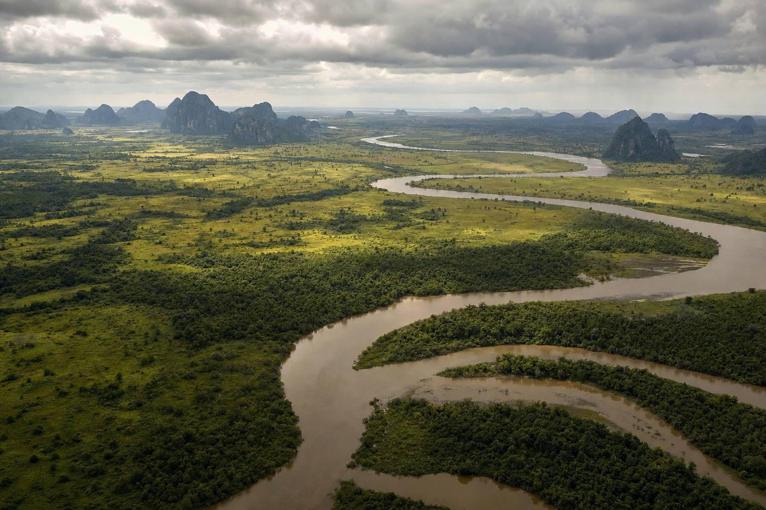
A lower sea redrew the map. In Southeast Asia, the shallow Sunda Shelf rose out of the water as a landmass called Sundaland, about twice the size of the land there today.
The Gulf of Thailand was dry land, crossed by rivers, joining the Malay Peninsula, Sumatra, Java and Borneo to Asia. A drop of just thirty to forty metres is enough. Try the sea-level buttons.
As the ice melted, the sea returned, flooding Sundaland step by step until about seven thousand years ago.
Where the sea is now A river plain of grass and forest on the dry shelf. AI-generated still.
~1.8 million km²
at its largest
30–40 m
lower sea joins the big islands to Asia
Sundaland
~21,000 years ago Whole shelf dry, sea ~120 m lower
~18,000 years ago Flooding begins
~7,000 years ago Coasts near today’s
The sea returns
Chapter II · The last great freeze
Sundaland
Wikipedia, Sundaland: at the Last Glacial Maximum sea level fell about 120 m and the entire Sunda Shelf was exposed; a drop of 30–40 m or more connected Borneo, Java and Sumatra to the Malay Peninsula and mainland Asia; the Gulf of Thailand lies within Sundaland, whose extent follows roughly the 120 m depth line; drowned river systems have been mapped on the shelf; it was partly submerged from about 18,000 years ago until about 5000 BC; its total area is about 1.8 million km², roughly twice the land there today.
Try the sea-level buttons. The exposed shelf is drawn approximately, not from a depth map.
The 3D scenes are simplified teaching models: the orbit is exaggerated, ice and coastlines are drawn approximately, and the curves are schematic unless a source is named.
But why would ice sheets grow and melt at all? In Glasgow, James Croll, a self-taught scientist working as a janitor at a college museum, looked to the sky.
Earth’s path around the Sun is not a perfect circle, and its shape slowly changes. Croll argued that when the orbit is more stretched, winters that fall when Earth is farthest from the Sun turn colder, so snow piles up.
He added a crucial idea: snow and ice reflect sunlight, so once they spread, they cool the planet further. Later work showed that cool summers matter more than cold winters, but the orbit and the ice feedback stayed.
A Victorian study A brass orrery and old astronomy books by lamplight. AI-generated still.
1821–1890
his life, in Scotland
1859
becomes janitor of the Andersonian museum
James Croll (Wikipedia)
A changing orbit alters the seasons
Bright snow reflects sunlight: cold makes more cold
Published in Climate and Time, 1875
Croll’s two ingredients
Croll: colder winters trigger ice ages
Later work: cool northern summers are the key
Kept: the orbit and the ice feedback
What lasted, and what did not
Chapter III · A wobbling orbit
James Croll
Wikipedia, James Croll (1821–1890): from 1859 he worked as janitor of the museum of the Andersonian University in Glasgow, using its library to teach himself physics and astronomy; he proposed that when Earth’s orbit is highly eccentric, winters that occur when Earth is farthest from the Sun are colder, favouring ice ages; he linked more snow to a positive feedback through reflective ice; his book Climate and Time, in Their Geological Relations appeared in London in 1875; he predicted ice ages alternating between the hemispheres roughly every 22,000 years, a pattern later evidence did not bear out, and he thought colder winters were the trigger, whereas later work pointed to cool summers.
The 3D scenes are simplified teaching models: the orbit is exaggerated, ice and coastlines are drawn approximately, and the curves are schematic unless a source is named.
Today we count three slow changes. The first is eccentricity, the shape of the orbit, which swings from nearly circular to slightly stretched and back over roughly a hundred thousand years.
Today the orbit is close to circular. Earth is about five million kilometres closer to the Sun in early January than in July, yet northern winters stay cold, because the tilt of the axis, not the distance, makes the seasons.
Over a whole year, the shape changes Earth’s total sunlight by well under one percent. Its real power, as we will see, is to make another cycle stronger or weaker.
~100,000
years per cycle
0.017
today: nearly a circle
Eccentricity (NASA)
5.1 million km
closer to the Sun in January
6.8%
more sunlight in January
January versus July (NASA)Sˉ∝1−e21
e
eccentricity: 0 for a circle; about 0.06 at most over the last million years, up to ~0.07 over longer spans
Sˉ
yearly average: only ~0.2% more at e = 0.06
Sunlight averaged over a year
Chapter III · A wobbling orbit
Eccentricity
NASA Science: the shape of Earth’s orbit varies over a cycle of about 100,000 years and is slowly becoming more circular; perihelion and aphelion now differ by about 5.1 million km, a 3.4% variation, and each January Earth receives about 6.8% more incoming solar radiation than in July; at maximum ellipticity about 23% more reaches Earth at perihelion than at aphelion. NASA Earth Observatory: the eccentricity is currently about 0.017. The yearly average follows from the geometry of an ellipse, a standard result: it scales as 1/√(1−e²), which is only about 0.2% higher at e = 0.06 than for a circle.
Try the buttons to change the orbit’s shape. The ellipse is drawn far more stretched than Earth’s real orbit so the change can be seen.
The 3D scenes are simplified teaching models: the orbit is exaggerated, ice and coastlines are drawn approximately, and the curves are schematic unless a source is named.
The second is obliquity, the tilt of Earth’s axis, which gives us our seasons. Over about forty-one thousand years, the tilt rocks between about twenty-two point one and twenty-four point five degrees.
More tilt means hotter summers and colder winters near the poles. Less tilt means cooler summers there, so some of the winter snow in the far north can survive until the next winter.
Today the tilt is about twenty-three point four degrees, and slowly shrinking.
~41,000
years per cycle
22.1°–24.5°
range over the last million years
Obliquity (NASA)
24.5°: sunnier summers, more melting
22.1°: cooler summers, snow survives
Try the buttons: the box shows midsummer sunlight
What tilt does at 65°N
~10,000 years ago Greatest tilt
Today 23.4°, decreasing
~10,000 years ahead Least tilt
The tilt now (NASA)
Chapter III · A wobbling orbit
Obliquity
NASA Science: the angle of Earth’s axis relative to its orbital plane has varied between 22.1° and 24.5° over the last million years, over a cycle of about 41,000 years; it is now about 23.4° and very slowly decreasing; it was at its maximum about 10,000 years ago and will reach its minimum about 10,000 years from now; decreasing tilt gives milder seasons and favours the build-up of ice sheets, as warmer winters hold more snow and cooler summers melt less of it.
The readout computes midsummer sunlight at 65°N from the tilt and the orbit with the standard formula for daily solar radiation at the top of the atmosphere; it is a simplified calculation, not a climate model.
The 3D scenes are simplified teaching models: the orbit is exaggerated, ice and coastlines are drawn approximately, and the curves are schematic unless a source is named.
The third is precession. Like a spinning top, Earth’s axis slowly traces a circle, about once every twenty-six thousand years, while the orbit itself slowly turns as well.
Together, they move the seasons around the orbit. On average every twenty-three thousand years, the point where Earth is closest to the Sun drifts through the whole calendar.
Right now Earth is closest to the Sun during the northern winter. In about thirteen thousand years that will flip, and northern summers will come when Earth is closest, so they will be sunnier. The more stretched the orbit, the bigger this effect.
25,771
years: the axis traces its circle
~112,000
years: the orbit itself turns once
Two motions (NASA)
~23,000
years, on average, for the seasons to cycle around the orbit
Together
Now: early January, northern winter
In ~13,000 years: northern summer
Effect is bigger when the orbit is more stretched
Closest to the Sun
Today
~478
Closest to the Sun in June (today’s orbit shape)
~510
Midsummer sunlight at 65°N (simple calculation)
Chapter III · A wobbling orbit
Precession
NASA Science: axial precession, the wobble of Earth’s rotation axis, has a cycle of about 25,771.5 years; apsidal precession, the slow turning of the orbit, about 112,000 years; combined, the climatic precession cycle averages about 23,000 years; perihelion now occurs during the Northern Hemisphere winter, and in about 13,000 years this flips, making seasonal contrasts more extreme in the north; eccentricity sets how strong the effect is.
Try the buttons to compare today with 13,000 years from now. The orbit is drawn exaggerated.
The 3D scenes are simplified teaching models: the orbit is exaggerated, ice and coastlines are drawn approximately, and the curves are schematic unless a source is named.
Adding the three up by hand was a huge task. It was taken on by the Serbian engineer and mathematician Milutin Milanković.
Even while interned during the First World War, he kept calculating, in a library in Budapest.
The climatologist Wladimir Köppen pointed him to the key: summer sunlight near sixty-five degrees north, where the great ice sheets grew. If those summers are cool, winter snow survives, and ice builds up year after year.
In 1941 he published his Canon of Insolation, with curves of sunlight reaching back six hundred thousand years. For decades, many geologists set it aside.
Sums by hand Pages of hand-written figures, a slide rule and a globe. AI-generated still.
1879 Born in Dalj
1914–1918 Interned; works in Budapest
1924 Köppen and Wegener print his curve
1941 Canon of Insolation, 626 pages
1958 Dies in Belgrade
Milanković’s life (EGU)
The great ice sheets grew near that latitude
Cool summers let snow last the year
Try the buttons to add each cycle to the curve
Why 65°N summers?
600,000
years of sunlight curves, before 1800
~50 years
before the idea was widely tested
The Canon (NASA Earth Observatory)
Chapter IV · Milanković’s sums
Milutin Milanković
European Geosciences Union: Milanković was born on 28 May 1879 at Dalj near Osijek, then in Austria-Hungary, and died on 12 December 1958 in Belgrade; interned at the start of the First World War, at Nezsider and later in Budapest, he was allowed to work in the library of the Hungarian Academy of Sciences; Wladimir Köppen and Alfred Wegener printed his insolation curve in 1924; his 626-page Canon of Insolation of the Earth and Its Application to the Problem of the Ice Ages was completed in 1941 and published by the Royal Serbian Academy. NASA Earth Observatory: Köppen suggested that he model summer insolation at 65°N, where great ice sheets grew; he calculated insolation for 600,000 years before 1800; the theory was largely ignored for about 50 years.
The curve on screen adds three waves of 23,000, 41,000 and 100,000 years to show the idea; it is schematic, not Milanković’s calculated curve.
The 3D scenes are simplified teaching models: the orbit is exaggerated, ice and coastlines are drawn approximately, and the curves are schematic unless a source is named.
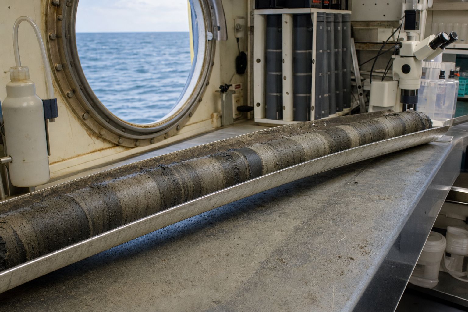
The proof came from the bottom of the sea. Tiny shelled plankton called foraminifera build their shells from seawater. The oxygen in those shells comes in a lighter and a heavier form.
Water with the lighter oxygen evaporates more easily, so the snow that builds ice sheets is rich in it. As ice grows, the ocean and the shells grow richer in the heavy kind, and the mud records how much ice there was on land.
In 1976 James Hays, John Imbrie and Nicholas Shackleton studied two cores from the southern Indian Ocean, spanning four hundred and fifty thousand years. Climate had swung with periods of twenty-three thousand, forty-two thousand and about a hundred thousand years.
Those were the orbit’s rhythms: the orbit, their paper said, is the pacemaker of the ice ages.
Foraminifera Chalky shells, each smaller than a grain of sand. AI-generated still.A sediment core Bands of deep-sea mud in a tray aboard ship. AI-generated still.
Light oxygen-16 evaporates more readily
Ice sheets lock it up on land
More heavy oxygen-18 in shells: more ice on land
Oxygen in a shell
Precession
23
Tilt
42
Eccentricity
~100
Rhythms found in the cores (Hays et al., 1976) 42,000 as measured in 1976; the tilt cycle is ~41,000 years.
Variations in the Earth’s Orbit: Pacemaker of the Ice AgesHays, Imbrie & Shackleton, Science, 10 December 1976
Chapter V · Proof in the mud
The pacemaker
Spencer Weart’s history of the discovery: Cesare Emiliani measured oxygen isotopes in foraminifera shells from sediment cores in 1955; work by Nicholas Shackleton showed that the signal mainly reflects the volume of ice on land, which holds more of the lighter isotope. Hays, Imbrie and Shackleton, Science 194 (1976): two cores, RC11-120 and E49-18, from the subantarctic southern Indian Ocean, gave a record of the past 450,000 years in which climatic variance is concentrated at periods of 23,000, 42,000 and approximately 100,000 years; their summary: “For 500,000 years, major climatic changes have followed variations in obliquity and precession.”
Press the button to split the schematic record into its rhythms.
The 3D scenes are simplified teaching models: the orbit is exaggerated, ice and coastlines are drawn approximately, and the curves are schematic unless a source is named.
There is a puzzle, though. The orbit mostly moves sunlight between seasons and latitudes. To build ice sheets kilometres thick, Earth must amplify that nudge.
One amplifier is the ice itself. Snow can reflect up to ninety percent of sunlight, while the open ocean reflects only about six percent. More ice means more sunlight bounced away, and more cooling.
Another is carbon dioxide. Air trapped in Antarctic ice shows that over eight hundred thousand years, carbon dioxide rose and fell with the ice ages, between about one hundred and seventy-two and three hundred parts per million.
Much of the missing carbon is thought to have gone into the deep ocean; exactly how is still being studied.
Snow, up to
90%
Bare sea ice
50–70%
Open ocean
6%
How much sunlight is reflected (SEOS)
Air from the past Bubbles of old air sealed inside an ice core. AI-generated still.
800,000
years of air in the ice
172–300
ppm: CO2 range before industry
EPICA Dome C (Lüthi et al., Nature, 2008)
74%
as much CO2 drawdown from cooling only the far north as from cooling the whole planet (idealized model)
One new idea (St Andrews ocean model, 2026)
Chapter VI · Amplifiers
Feedbacks
SEOS: the albedo of bare sea ice is about 0.5 to 0.7, snow has an even higher albedo of up to 0.9, and a typical ocean albedo is 0.06. Lüthi and colleagues, Nature 453 (2008): measurements from the EPICA Dome C ice core extended the CO2 record to 800,000 years and reported the lowest value yet found in an ice core, 172 parts per million; the late-Quaternary range before industry is 172–300 ppm. ScienceDaily (28 October 2026): the St Andrews model proposes that cooling of the North Atlantic by growing ice sheets spreads south and changes circulation around Antarctica, letting the ocean store more CO2 below the surface; it is a model result, not a confirmed cause.
Try the buttons to cover the scene with ice or open sea and see how much sunlight is reflected. The CO2 curve on screen is schematic in shape; its range is from the ice core.
The 3D scenes are simplified teaching models: the orbit is exaggerated, ice and coastlines are drawn approximately, and the curves are schematic unless a source is named.
Not everything is solved. In the early part of the Quaternary, ice ages came about every forty-one thousand years, in step with the tilt.
Then, about one point two million years ago, the rhythm slowed to roughly a hundred thousand years, a change called the Mid-Pleistocene Transition, whose cause is still debated.
The orbit kept its rhythms, so the answer probably lies in how Earth itself responded, perhaps through several causes at once.
Early Pleistocene
~41
Last ~1.2 million years
~100–120
How long one ice-age cycle lasts (Eos, 2021)
~1.2 million
years ago: longer cycles begin
Unknown
cause, still debated
Pleistocene
the Quaternary before the Holocene
The Mid-Pleistocene Transition
Slow global cooling
Bigger ice sheets that outlast warm summers
Ice scraping soil down to bedrock
Probably several at once
Ideas being tested (Eos, 2021)Scraped to bedrock Bare, ice-smoothed bedrock where soil was stripped away. AI-generated still.
Chapter VI · Amplifiers
An open question
Eos (2021), by C. J. Berends, R. van de Wal and L. J. Lourens, on their review in Reviews of Geophysics: during the Early Pleistocene, ice-age cycles lasted about 41,000 years, matching the obliquity cycle; for the past 1.2 million years they have lasted roughly 100,000 to 120,000 years; how a 41,000-year orbital rhythm can lead to a 100,000-year response is unresolved, and the evidence is limited; hypotheses include gradual global cooling with non-linear ice-sheet feedbacks, and the erosion of soil under the ice sheets; several mechanisms likely contributed.
Try the buttons to highlight the 41,000-year era and the 100,000-year era on the schematic curve.
The 3D scenes are simplified teaching models: the orbit is exaggerated, ice and coastlines are drawn approximately, and the curves are schematic unless a source is named.
So what about today? The orbital cycles work over tens of thousands of years. Today’s warming has happened over decades, far too fast for the orbit to explain.
Carbon dioxide measured at Mauna Loa in Hawaii peaked at about four hundred and thirty-two parts per million in May 2026, far above the whole eight-hundred-thousand-year ice record, and the rise is caused by people.
Left to itself, the orbit would now be nudging Earth very slowly towards cooling, not warming. The ice ages teach one lesson that still matters: a small push, amplified by ice and carbon dioxide, can remake the planet.
Lowest in the ice (glacial)
172
Highest in the ice, before industry
300
Mauna Loa, May 2026
432
Carbon dioxide, parts per million
Orbital cycles: tens of thousands of years
Today’s warming: decades
Orbit alone would now favour slow cooling
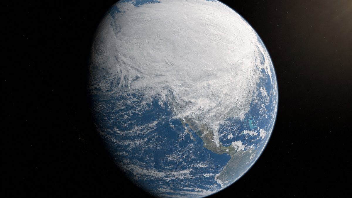
Two clocks (NASA)One planet, one orbit Earth with its polar ice, lit by the Sun. AI-generated still.
1837 Agassiz: an ice age
1875 Croll: orbit and ice feedback
1941 Milanković’s Canon
1976 Pacemaker of the Ice Ages
2008 800,000 years of CO2 in ice
2026 432 ppm at Mauna Loa
How we learned it
Epilogue
Why today is different
NASA Science: Milankovitch cycles act over tens to hundreds of thousands of years, while current warming has happened over decades to centuries; incoming sunlight has increased only slightly over the past century; Earth is now in an interglacial, and orbital factors would favour cooling, not warming. UC San Diego and Scripps (2026): carbon dioxide at Mauna Loa peaked at 432.0 ppm in May 2026 (NOAA: 432.3 ppm), the most important human-caused greenhouse gas; Keeling’s record began at 313 ppm in 1958. Lüthi et al. (2008): the range in the 800,000-year ice core record before industry is 172–300 ppm. All facts in this film come from the sources listed in each panel. The 3D scenes are simplified teaching models and the still images are AI-generated.
Press the button to add 2026 to the schematic ice-core curve.
The 3D scenes are simplified teaching models: the orbit is exaggerated, ice and coastlines are drawn approximately, and the curves are schematic unless a source is named.